
Decision Tree in Machine Learning: How It Works
Introduction
A decision tree in machine learning makes a prediction by moving an example through a sequence of feature-based tests. At each step, a condition sends the example along a branch; the final branch leads to an output, such as a category or a number. The process resembles following a flowchart, but the model’s decision rules are learned from training data rather than written out by hand for every prediction.
Understanding that path makes the model easier to evaluate. The sections below explain the tree’s structure, how training selects splits, and how a sample reaches a prediction. They also cover why a compact tree can be straightforward to inspect, why a very complex one can be harder to follow, and what to consider when choosing or evaluating this model.
What Is a Decision Tree in Machine Learning?
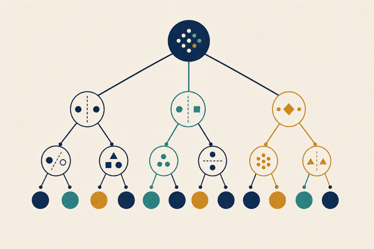
A decision tree is a model organized as a set of connected tests. It has a root node, where a path begins; internal nodes, which test a feature or condition; branches, which represent the possible outcomes of a test; and leaf nodes, which end a path and provide an output. Scikit-learn describes tree training as repeatedly choosing a split and applying the process to the resulting groups until a stopping condition is met (documentation).
For example, an internal node might test whether a measurement is below a threshold. One branch represents “yes,” the other “no.” Each branch can lead to another test or to a leaf. The exact tests and branch structure depend on the tree learned during training.
A route from the root to a leaf is a sequence of decisions. The complete collection of nodes and branches is the model’s learned structure; a prediction is the result of applying that structure to one particular input. Because branch choices depend on feature values, two inputs can follow different routes through the same fitted tree and arrive at different leaves. The model remains the same; only the path taken for each prediction changes. A small tree’s explicit tests and paths can be inspected, though larger trees may be difficult to follow (tree-structure guide).
How a Decision Tree Makes Decisions
To make a prediction, the model starts at the root and checks the input against that node’s test. The result determines which branch to follow. At the next node, another feature test may narrow the route further. This continues until the example reaches a leaf, where the tree returns its prediction. Scikit-learn documents decision paths and leaf identifiers for tracing how samples move through a fitted tree (tree-structure guide).
Illustrative path, not a real dataset:
Root: Is feature A below the learned threshold?
├── Yes: Is feature B above its learned threshold?
│   ├── Yes → Leaf: Category 1
│   └── No  → Leaf: Category 2
└── No  → Leaf: Category 3
An input that answers “yes” at the root and “no” at the next test follows the highlighted route in effect: root → left branch → second test → its “no” branch → Category 2 leaf. The example shows the mechanics only; its features, thresholds, and categories are hypothetical.
The path is conditional, not a checklist that every input follows in full. A later test is reached only when the earlier branch outcomes lead to it, so different inputs can take different routes and end at different leaves. For a fitted tree, the learned tests and branch structure determine which route an input follows.
The tests are part of the trained model. A user supplies features, and the fitted tree applies its learned rules; the user does not normally hand-write a separate chain of decisions for each input. In a classification task, the leaf supplies a category prediction. In scikit-learn’s classifier, class probabilities at a reached leaf are based on the training samples there, and the predicted class is the one with the highest probability (classifier documentation). That is an implementation-specific description, not a rule to assume for every library.
A route is also a compact way to describe why the model returned an output: it exposes the tests encountered for that input. This can make a small tree easier to inspect, but does not guarantee that every tree, especially a large one, will be easy for people to understand.
How the Tree Learns Its Splits
During training, the algorithm uses examples with known outcomes to build the tree. At a node, it considers possible feature-based splits and selects one according to a task-specific objective. The split divides the examples into child groups; the process can then repeat within those groups until a stopping condition is reached. This recursive procedure is documented for scikit-learn, though search strategies and options can differ among implementations (decision-tree documentation).
A split criterion measures how useful a candidate division is for the learning objective. In classification, the aim is to form groups that are more informative about the target classes; in regression, the criterion relates to numerical prediction error. For scikit-learn classification trees, available criteria include Gini impurity, entropy, and log loss (classifier documentation). These are options in that implementation, not universally required or proven best choices.
Conceptually, the criterion gives the learner a way to compare candidate divisions: it evaluates how well the resulting groups serve the task, rather than choosing a split simply because it creates more branches. The selected split is useful relative to the chosen objective, but that does not by itself establish how well the finished tree will perform on new examples.
The algorithm evaluates candidate features and, where relevant, thresholds according to its procedure. It does not follow that every tree implementation tests every possible threshold in the same way. The chosen split is followed by further splits, subject to the model’s stopping rules. In scikit-learn regression trees, the selected criterion also affects terminal-node output: squared error and Poisson use a mean, while absolute error uses a median (regression example). Leaf behavior therefore depends on the task, criterion, and implementation.
A Simple Decision Tree Example
Imagine a hypothetical decision tree that predicts whether a student will pass a course. It uses two features: weekly study hours and a practice-quiz score. The values and outcomes below are fictional and are included only to show how a prediction follows a path through a tree.
The root test asks whether the student studies at least three hours per week. This is the first decision point. The tree has two branches: one for “yes” and one for “no.” If the answer is “no,” the path ends at a leaf labeled “not predicted to pass.” If the answer is “yes,” the next test asks whether the practice-quiz score is at least 70. That test also has two branches, leading to a leaf labeled either “predicted to pass” or “not predicted to pass.”
Suppose a hypothetical student studies 4.5 hours per week and scores 82 on the practice quiz. The first test is true, so the path follows the “yes” branch. The second test is also true, so the path reaches the “predicted to pass” leaf. The tree returns that leaf’s output; it does not continue evaluating other branches for this example.
This simplified illustration shows how feature tests route an input to a prediction leaf, as in the documented tree structure. It leaves out the details of choosing splits and training a model on real data, and its prediction is not evidence about actual student outcomes.
Decision Trees for Classification and Regression
A decision tree can predict either a category or a numerical value, depending on the task. Classification assigns an input to a class, such as “pass” or “not predicted to pass.” Regression predicts a number, such as a hypothetical delivery time in minutes. In both cases, the input follows tests down the tree to a leaf, but the leaf’s output is suited to the task.
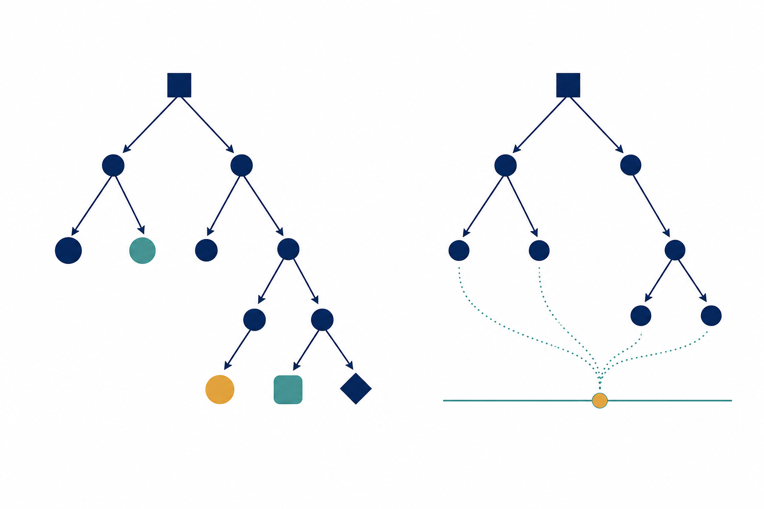
The exact output rule depends on the implementation and its chosen criterion. In scikit-learn, a classifier associates class probabilities with each reached leaf and predicts the class with the highest probability. For regression, scikit-learn documents criteria where terminal nodes use a mean, as well as an absolute-error criterion that uses a median. These are implementation-specific examples, not rules that apply to every tree library.
| Task | Prediction type | Illustrative leaf output |
|---|---|---|
| Classification | Category or class | “Pass” |
| Regression | Numerical value | 42 minutes |
The examples are illustrative. See the scikit-learn classification documentation and its regression example for details on those implementation-specific outputs.
This distinction is useful when reading a model’s output: a class label answers which category is selected, while a regression value gives a quantity on the target’s numerical scale. The table’s examples are illustrative rather than recommended thresholds or expected predictions. The criteria determine how a regression leaf summarizes its training examples; therefore, a mean is not a universal rule.
Overfitting and Controlling Tree Complexity
A tree can keep adding branches to fit distinctions in its training data. If it grows complex enough to capture patterns specific to those examples, it may not make equally useful predictions on new data. This is the risk of overfitting: a close fit to the training set alone does not show that the model will generalize well.
One way to manage complexity is to limit growth. Scikit-learn documents controls including maximum depth, minimum samples required for a split, minimum samples per leaf, and a minimum impurity decrease. Pruning takes a different approach by removing parts of a grown tree; scikit-learn describes minimal cost-complexity pruning as a method for pruning a tree to avoid overfitting. These are tools to consider, not guaranteed improvements. The useful settings depend on the data and should be assessed with an appropriate validation approach.
These controls act at different points: a depth cap limits how many levels the tree can add, while minimum-sample rules require enough observations to support a split or leaf. A minimum impurity-decrease threshold can prevent splits that make too little improvement under the chosen criterion. Compare candidate settings using validation data suited to the task; the best balance is dataset-dependent, not inferable from training fit alone.
A tree that fits its training data closely has not, by that fact alone, demonstrated strong performance on unseen examples.
The scikit-learn tree guide documents these complexity controls and pruning. It does not establish one setting as optimal for every dataset.
Strengths, Limitations, and When to Consider a Decision Tree
A small tree can be inspected as a sequence of feature tests and branches, which makes its decision path explicit. That structure may help when people need to examine how a prediction was reached. It does not mean every tree is easy to interpret: as branches accumulate, following the full structure can become difficult.
A single tree can also be sensitive to its training data. A study of single-tree classification methods describes how small data changes can alter early split decisions, with effects that propagate as the tree grows. The degree of instability can depend on the data and evaluation, so it should not be assumed to have the same impact in every setting.
Consider a decision tree in light of the task, the data, how predictions will be evaluated, and how important an inspectable model is. A small tree’s explicit path may be useful, but its complexity and sensitivity are relevant trade-offs. The tree-structure example illustrates the inspectable form, while the study on classification-tree stability discusses sensitivity in single-tree methods.
Conclusion
A decision tree makes a prediction by following feature-based tests from its root to a leaf. Training determines the tests and the tree’s structure; the leaf supplies the output for the task. When assessing a model, consider whether its classification or regression task fits your needs, how complex the tree has grown, and how it performs on validation data. Depth limits, sample thresholds, or pruning can help control complexity, but their effects depend on the data and tuning. For ongoing AI and technology context, you can Subscribe Free to The Deep View Newsletter.
Summary
Learn how a decision tree in machine learning routes inputs through feature-based tests to produce category or numerical predictions. The article explains how trees learn splits, how complexity and overfitting are managed, and what to consider when evaluating their interpretability and performance.